Cosmos WFM (1/3): Foundations — World Models, Data, and Tokenization
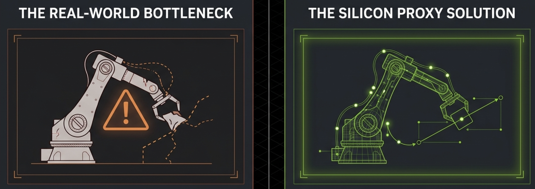
TL;DR: Physical AI — robots, self-driving cars, humanoids — can’t scale by training in the real world alone. A World Foundation Model (WFM) is a learned video simulator: given past frames and a perturbation, it predicts the visual future. Training such a model requires industrial-scale data curation (35M hours → 200M clips, 4% survival rate) and video tokenization that compresses raw frames into compact tokens a transformer can process — either continuous (for diffusion) or discrete (for autoregressive models).
These paper reviews are written more for me and less for others. LLMs have been used in formatting
This is Part 1 of a 3-part series on NVIDIA’s Cosmos World Foundation Models, drawing from two papers: Cosmos World Foundation Model Platform for Physical AI (2025) and World Simulation with Video Foundation Models for Physical AI (2026).
The Problem with Real-World Training
Physical AI — robots, autonomous vehicles, embodied agents — learns by interacting with the environment. Sensors observe, actuators act, and the system updates its policy based on what happened. Simple enough in principle. In practice:
- It is slow. A robot arm practising grasping takes thousands of real-world hours.
- It is expensive. Hardware wears out. Environments must be instrumented.
- It is dangerous. Early-stage policies are bad policies. A self-driving car exploring edge cases on public roads is not a good idea.
- Data is hard to scale. Unlike language or images, Physical AI data requires interleaved sequences of observations and actions. You cannot just scrape them from the internet.
The core bottleneck: scaling training data for Physical AI is fundamentally harder than for language or vision.
What Is a World Foundation Model?
A WFM is a digital twin of the physical world — a model that, given past observations and a perturbation, predicts what happens next.
Formally: let $x_{0:t}$ be a sequence of visual observations (video frames) from time $0$ to $t$. Let $c_t$ be a perturbation — an action, a text description, or a random disturbance. A WFM $\mathcal{W}$ generates:
\[\hat{x}_{t+1} = \mathcal{W}(x_{0:t},\ c_t)\]The perturbation $c_t$ is what makes this a world model rather than just a video predictor. It gives control — you can ask “what happens if the robot arm moves left?” and the WFM generates the corresponding visual future.
If the WFM is good enough, the agent can train entirely inside the simulation. No real-world damage, no hardware cost, unlimited data.
What Can You Do with a WFM?
Five concrete use cases:
Policy evaluation. Let a trained robot policy interact with the WFM instead of the real world. Generate rollouts, observe failures, rule out bad policies before committing physical resources.
Policy initialisation. A WFM that has learned world dynamics — how objects move, how gravity works, how materials deform — contains a rich physics prior. This prior can initialise the policy model, addressing data scarcity.
Policy training. Pair a WFM with a reward model and you have an RL environment. The agent takes actions, the WFM generates the next state, the reward model scores it. A physics simulator learned from data rather than hand-coded.
Planning. Simulate multiple future trajectories under different action sequences. A cost function scores each outcome. The agent picks the best plan.
Synthetic data generation. Fine-tune the WFM on rendering metadata (depth maps, segmentation masks) and use it as a conditional generator. Take a physics simulator’s simple output and translate it into photorealistic video for training perception models.
The Pre-train / Post-train Paradigm
Cosmos follows the same two-stage recipe that has worked for LLMs:
Pre-training produces a generalist. Train on a massive, diverse video dataset — driving, object manipulation, human motion, nature, spatial navigation — so the model learns general physics and visual dynamics.
Post-training produces a specialist. Fine-tune on a smaller, task-specific dataset — robotic manipulation videos, driving clips from a specific sensor rig, factory floor scenarios. The pre-trained model already knows physics; post-training teaches it your specific setup.
This is efficient because pre-training is done once and amortised across all downstream applications, and post-training datasets can be small because the model already has a strong prior.
Curating the Training Data
A world model trained on raw internet video would learn to generate YouTube editing artefacts, not physics. Raw video is full of shot transitions, overlays, visual effects, low quality, and redundancy. The data pipeline’s job is to extract the subset that teaches the model about how the physical world actually works.
Cosmos processes 35 million hours of raw video through a seven-stage pipeline. Only 4% survives.
1. Shot-aware splitting. Segment long videos into single-shot clips. A world model should not learn to predict a jump cut — those are editorial, not physical.
2. Transcoding. Re-encode everything into a uniform high-quality format. Consistency matters at scale.
3. Cropping. Remove black borders and spatial padding.
4. Filtering. This is the critical stage — six sequential filters targeting different quality dimensions:
- Aesthetic quality — visual appeal (learned scorer, not rule-based)
- Motion — remove static or random-jitter video; tag remaining clips by motion type
- Text overlay — remove clips with excessive post-production text (titles, watermarks, subtitles)
- Perceptual quality — remove noisy, blurry, over/underexposed content
- Semantic artefacts — catch video-in-video, animations, cartoons, game footage — visually “fine” but not real-world physics
- VLM filter — a vision-language model does a final high-precision pass, catching subtle issues the specialised classifiers miss
5. Captioning. Each surviving clip gets a text description from a VLM. These captions serve as the supervision signal during training and the conditioning prompt at inference.
6. Semantic deduplication. Cluster video embeddings, find near-duplicates within clusters, keep the highest-resolution version. About 30% of clips are removed here.
7. Sharding. Package clips into structured datasets by content type, resolution, aspect ratio, and length — enabling curriculum learning and domain balancing during training.
Tokenizing Video
A single second of 720p video at 16 fps contains roughly 43 million pixel values. A transformer cannot process this directly. Video must be compressed into a compact sequence of tokens — an encoder-decoder pair where the encoder compresses and the decoder reconstructs.
Continuous vs Discrete Tokens
Continuous tokens are dense vectors in $\mathbb{R}^C$, produced by a standard autoencoder. Used by diffusion models, which operate in continuous latent space.
Discrete tokens are integers from a finite vocabulary, produced by a quantized autoencoder. Used by autoregressive models, which predict the next token like GPT predicts the next word.
For discrete tokenization, Cosmos uses Finite-Scalar-Quantization (FSQ). FSQ maps each dimension of the latent vector to a finite set of levels. With a 6-dimensional latent and levels $(8, 8, 8, 5, 5, 5)$, the vocabulary is $8^3 \times 5^3 = 64{,}000$ tokens. FSQ avoids the codebook collapse problem of traditional VQ-VAE while being simpler.
Causality
Every operation respects temporal causality — tokens for frame $t$ never depend on frame $t+1$. This matters for two reasons:
- Joint image-video training: an image is just a video of length 1, and the causal structure handles it naturally
- Deployment: Physical AI systems process video in real time — a causal tokenizer can stream without buffering future frames
Compression
Tokens span spatial ($H/s_{HW} \times W/s_{HW}$) and temporal ($1 + T/s_T$) dimensions. Cosmos trains tokenizers at multiple compression rates — from gentle ($4 \times 8 \times 8$, preserving detail) to aggressive ($8 \times 16 \times 16$, 2048x total compression). Higher compression saves compute but loses detail.
Architecture and Training
The encoder applies a 3D Haar wavelet transform (separating frequency bands, analogous to JPEG but learned end-to-end and extended to the temporal dimension), followed by causal residual blocks with factorised 3D convolutions and causal attention for long-range dependencies. The decoder mirrors this structure.
Training uses a multi-loss strategy across two stages:
- Stage 1: L1 reconstruction loss + VGG-19 perceptual loss (match structure, not just pixels)
- Stage 2: add optical flow loss (temporal smoothness) + Gram-matrix loss (texture sharpness) + adversarial loss
What Is Coming in This Series
- Part 2 — Training: Diffusion vs autoregressive world models, flow matching, and post-training recipes (model merging, RL, distillation).
- Part 3 — Applications: Sim2Real, robot policy augmentation, action-conditioned generation, and multi-view simulation.
Key Takeaways
- Physical AI cannot scale by training in the real world alone — it is too slow, expensive, and dangerous.
- A WFM is a learned video simulator: given past frames + a perturbation, it predicts the visual future.
- WFMs enable policy evaluation, training, planning, and synthetic data generation without real hardware.
- Cosmos follows the pre-train (generalist) → post-train (specialist) paradigm, same as LLMs.
- Data curation is aggressive: 35M hours → 200M clips, only 4% survive six filtering stages.
- Video tokenization compresses frames into continuous (for diffusion) or discrete (for autoregressive) tokens via a causal encoder-decoder.
- FSQ provides a 64K-token vocabulary for discrete tokenization without codebook collapse.
- Multi-stage training losses (L1, perceptual, flow, Gram, adversarial) balance reconstruction fidelity, temporal smoothness, and visual sharpness.