From Autoencoders to VAEs: Learning to Generate, Not Just Compress

TL;DR: Hinton’s autoencoder taught networks to compress data into a small latent vector and reconstruct it back. It worked beautifully — but the latent space was a mess you couldn’t generate from. Kingma & Welling’s VAE fixed this with one elegant shift: encode to a distribution, not a point. That single change turned a compression tool into a generative model.

These paper reviews are written more for me and less for others. LLMs have been used in formatting

---

The Problem: High-Dimensional Data is Redundant

Why Compress at All?

A 28×28 grayscale image is a vector in $\mathbb{R}^{784}$. But most of that 784-dimensional space is empty — natural images don’t live everywhere, they live on a low-dimensional manifold inside that space. A face, for instance, is defined by maybe a dozen meaningful factors: lighting, pose, expression, identity. The rest is just pixel-level detail.

If we could find that low-dimensional structure — the latent space — we’d have something powerful:

• Compression: represent data efficiently
• Denoising: project to manifold, reconstruct clean version
• Generation: sample from the latent space, decode into new data
• Interpolation: walk through latent space smoothly between two points

The question is how to learn that structure from data.

---

Hinton’s Autoencoder: Learning to Compress

The 2006 Paper

Hinton & Salakhutdinov’s Reducing the Dimensionality of Data with Neural Networks (Science, 2006) showed that deep neural networks could learn compact representations — better than PCA — by training them to reconstruct their own input.

The architecture is almost embarrassingly simple:

graph LR
    x["Input x<br/>784-dim"] --> e1["Encoder Layer 1<br/>512"]
    e1 --> e2["Encoder Layer 2<br/>256"]
    e2 --> z["Latent Code z<br/>32-dim 🗜️"]
    z --> d1["Decoder Layer 1<br/>256"]
    d1 --> d2["Decoder Layer 2<br/>512"]
    d2 --> xhat["Reconstruction x̂<br/>784-dim"]

    style z fill:#e3f2fd,stroke:#1976d2,stroke-width:2px,color:#000

• Encoder $f_\phi$: maps input $x$ to a compressed code $z$
• Decoder $g_\theta$: maps the code $z$ back to a reconstruction $\hat{x}$
• Bottleneck: the narrow middle layer forces compression

The Objective

Train to minimise reconstruction error:

\[\mathcal{L}_{AE} = \| x - \hat{x} \|^2 = \| x - g_\theta(f_\phi(x)) \|^2\]

That’s it. No labels needed — the target is the input itself. This is self-supervised learning before the term existed.

What the Latent Space Learns

This is the beautiful part. The network has no choice but to learn structure. If the bottleneck is 32-dimensional and the input is 784-dimensional, the encoder must throw away everything that isn’t essential. What survives is the semantics — the factors that actually matter for reconstruction.

Trained on faces, the latent space organises by lighting, pose, identity. Trained on digits, it organises by digit class, thickness, slant. No one told it to — it emerged from the reconstruction pressure.

The Problem: The Latent Space is a Mess

Here’s what nobody talks about enough. The autoencoder learns to compress the training data well. But the latent space has no global structure — it’s a collection of islands.

graph TD
    subgraph "Autoencoder Latent Space"
        A(["cluster: 3s"])
        B(["cluster: 7s"])
        C(["cluster: 1s"])
        gap1[" "]
        gap2[" "]
    end
    A ~~~ gap1
    gap1 ~~~ B
    B ~~~ gap2
    gap2 ~~~ C

Points between clusters map to nothing recognisable. Sample a random point from the latent space and decode it — you get garbage. The autoencoder learned to encode and decode, but it never learned to fill the space meaningfully.

You can’t generate from it. You can’t interpolate smoothly. The manifold is there, but it’s fragmented.

This is the problem VAEs solve.

---

Variational Autoencoders: Encoding to a Distribution

The 2013 Paper

Kingma & Welling’s Auto-Encoding Variational Bayes (2013) reframed the problem entirely. Instead of asking “what point in latent space represents this input?”, they asked:

“What distribution over latent space is consistent with this input?”

The encoder no longer outputs a single vector $z$. It outputs the parameters of a Gaussian — a mean $\mu$ and a variance $\sigma^2$.

\[q_\phi(z | x) = \mathcal{N}(z; \mu_\phi(x), \sigma^2_\phi(x))\]

Then $z$ is sampled from that distribution, and the decoder reconstructs from the sample.

graph LR
    x["Input x"] --> enc["Encoder f_φ"]
    enc --> mu["μ(x)"]
    enc --> sig["σ²(x)"]
    mu --> sample["Sample z ~ N(μ, σ²)"]
    sig --> sample
    sample --> dec["Decoder g_θ"]
    dec --> xhat["Reconstruction x̂"]

    style sample fill:#e8f5e8,stroke:#2e7d32,stroke-width:2px,color:#000
    style mu fill:#fff3e0,stroke:#f57c00,stroke-width:2px,color:#000
    style sig fill:#fff3e0,stroke:#f57c00,stroke-width:2px,color:#000

Why This Fixes the Latent Space

By encoding to a distribution rather than a point, the VAE is forced to make nearby regions of latent space decode to similar things. The variance $\sigma^2$ acts as a regulariser — if the encoder tries to collapse to a point (variance → 0), the KL term in the loss penalises it.

The result: a continuous, smooth latent space where you can sample anywhere and get something meaningful.

The VAE Loss: Two Terms

The VAE loss — derived from the Evidence Lower Bound (ELBO) — has two parts:

\[\mathcal{L}_{VAE} = \underbrace{\mathbb{E}_{q_\phi(z|x)}[\log p_\theta(x|z)]}_{\text{Reconstruction loss}} - \underbrace{D_{KL}(q_\phi(z|x) \| p(z))}_{\text{KL divergence}}\]

Reading it left to right:

• Reconstruction loss: on average over samples of $z$, how well does the decoder reconstruct $x$? This is the same pressure as the standard autoencoder.
• KL divergence: how far is the encoder’s distribution $q_\phi(z\vert x)$ from the prior $p(z) = \mathcal{N}(0, I)$? This term forces the latent space to stay close to a standard Gaussian — no wild clusters, no holes.

The two terms are in tension. Reconstruction wants the encoder to be precise (low variance, sharp encoding). KL wants the encoder to stay spread out (high variance, close to prior). The network learns to balance them.

Intuition: Reconstruction loss says “encode accurately.” KL divergence says “but not so accurately that you create islands.” The VAE learns representations that are both faithful and smooth.

The Reparameterisation Trick

There’s a subtle problem. The loss involves sampling $z \sim \mathcal{N}(\mu, \sigma^2)$, and sampling is not differentiable — you can’t backpropagate through a random node.

Kingma & Welling’s fix is elegant. Instead of sampling $z$ directly, rewrite it as:

\[z = \mu + \sigma \cdot \epsilon, \quad \epsilon \sim \mathcal{N}(0, I)\]

Now $\epsilon$ is the randomness — a fixed sample from a standard Gaussian. The parameters $\mu$ and $\sigma$ are deterministic functions of $x$. Gradients flow through $\mu$ and $\sigma$ cleanly, and $\epsilon$ is just noise.

graph LR
    x["x"] --> enc["Encoder"]
    enc --> mu["μ"]
    enc --> sig["σ"]
    eps["ε ~ N(0,I)"] --> z
    mu --> z["z = μ + σε"]
    sig --> z
    z --> dec["Decoder"]
    dec --> xhat["x̂"]

    style eps fill:#f3e5f5,stroke:#7b1fa2,stroke-width:2px,color:#000
    style z fill:#e8f5e8,stroke:#2e7d32,stroke-width:2px,color:#000

The randomness is moved outside the computation graph. This is the trick that makes VAEs trainable end-to-end.

---

PyTorch Implementation

A minimal VAE — encoder, reparameterisation, decoder, loss — in one clean block:

import torch
import torch.nn as nn
import torch.nn.functional as F

class VAE(nn.Module):
    def __init__(self, input_dim=784, hidden_dim=512, latent_dim=32):
        super().__init__()
        # Encoder
        self.fc1 = nn.Linear(input_dim, hidden_dim)
        self.fc_mu = nn.Linear(hidden_dim, latent_dim)
        self.fc_logvar = nn.Linear(hidden_dim, latent_dim)  # log σ² for stability
        # Decoder
        self.fc3 = nn.Linear(latent_dim, hidden_dim)
        self.fc4 = nn.Linear(hidden_dim, input_dim)

    def encode(self, x):
        h = F.relu(self.fc1(x))
        return self.fc_mu(h), self.fc_logvar(h)

    def reparameterise(self, mu, logvar):
        std = torch.exp(0.5 * logvar)   # σ = exp(log σ² / 2)
        eps = torch.randn_like(std)     # ε ~ N(0, I)
        return mu + std * eps           # z = μ + σε

    def decode(self, z):
        h = F.relu(self.fc3(z))
        return torch.sigmoid(self.fc4(h))

    def forward(self, x):
        mu, logvar = self.encode(x)
        z = self.reparameterise(mu, logvar)
        return self.decode(z), mu, logvar


def vae_loss(recon_x, x, mu, logvar):
    # Reconstruction: binary cross-entropy pixel-wise
    recon_loss = F.binary_cross_entropy(recon_x, x, reduction='sum')
    # KL divergence: closed form for N(μ,σ²) vs N(0,I)
    kl_loss = -0.5 * torch.sum(1 + logvar - mu.pow(2) - logvar.exp())
    return recon_loss + kl_loss

A few things worth noticing:

• We predict logvar (log variance) instead of variance directly — avoids numerical issues with negative values
• The KL divergence has a closed form when both distributions are Gaussian (see Appendix)
• reparameterise is three lines — that’s all the trick is

---

What VAEs Unlocked

1. Generation

Sample $z \sim \mathcal{N}(0, I)$, decode. Because the latent space is smooth and continuous, you get coherent outputs everywhere — not just at training points.

2. Interpolation

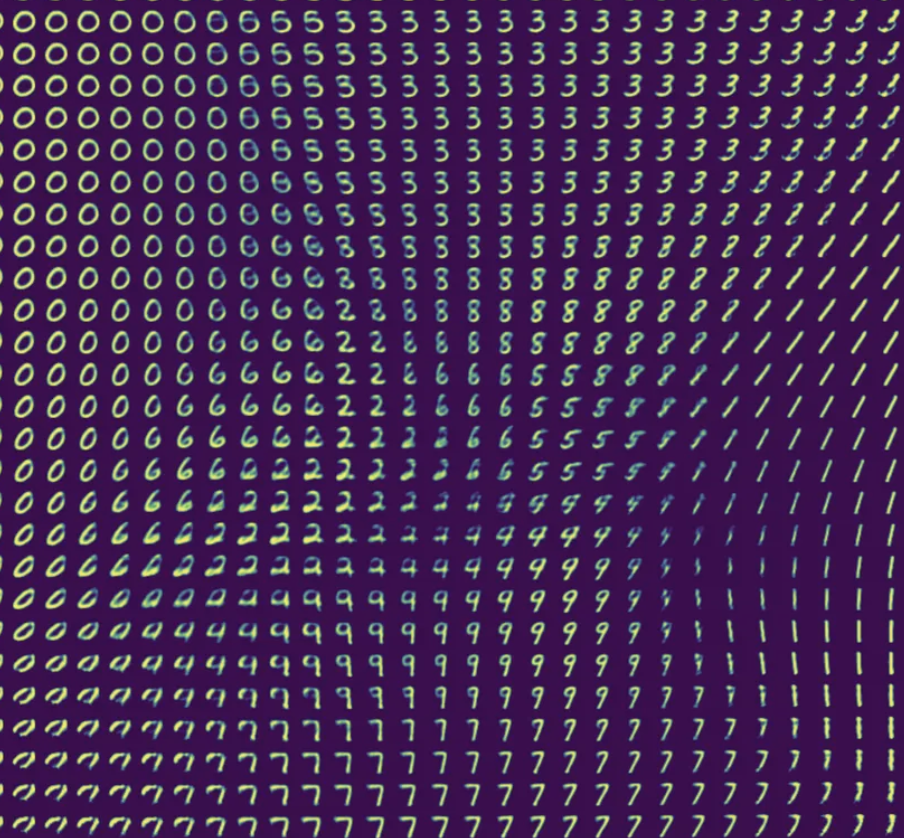
Take two images $x_1$ and $x_2$. Encode both to $\mu_1, \mu_2$. Linearly interpolate between them and decode each point. Because the latent space is smooth, the interpolation passes through meaningful intermediate states — not garbage.

3. Disentanglement

With the right training pressures (e.g. $\beta$-VAE), individual dimensions of $z$ learn to control individual factors of variation — one dimension for lighting, another for pose. Manipulating a single latent dimension changes one attribute without touching others.

---

The Honest Limitations

Issue	What Happens	Why
Blurry reconstructions	Generated images look soft and smeared	Reconstruction loss averages over all valid decodings of a $z$
Posterior collapse	Decoder ignores $z$ entirely	KL term can “win” — encoder collapses to prior, decoder memorises
Limited expressiveness	Can’t capture very complex distributions	Gaussian assumption in both encoder and prior is restrictive

The blurriness problem in particular held VAEs back from image generation. GANs, which came shortly after, produced sharper images by replacing the reconstruction loss with an adversarial discriminator. Diffusion models later solved it more cleanly. But VAEs remain the cleaner theoretical framework — principled, tractable, and interpretable.

---

The Lineage

timeline
    title From Autoencoders to Modern Generative Models
    2006 : Hinton & Salakhutdinov
         : Deep autoencoders beat PCA at compression
    2013 : Kingma & Welling
         : VAE — encode to distribution, structured latent space
    2014 : Goodfellow et al.
         : GAN — adversarial generation, sharper images
    2016 : β-VAE
         : Disentangled representations via KL weighting
    2020 : VQ-VAE-2
         : Discrete latent spaces, high-fidelity generation
    2021 : Diffusion Models
         : Score-based generation, VAE-style latent spaces
    2022 : Stable Diffusion
         : Latent diffusion in VAE latent space

Note that last entry: Stable Diffusion runs its diffusion process in the latent space of a VAE. The VAE is doing the compression; the diffusion model is doing the generation. Kingma & Welling’s 2013 latent space is powering images you’re looking at today.

---

Summary

flowchart TD
    A["Data lives on a low-dim manifold"] --> B["Autoencoder: learn to compress & reconstruct"]
    B --> C["Problem: latent space is unstructured — can't generate"]
    C --> D["VAE: encode to a distribution q(z|x)"]
    D --> E["KL divergence forces smooth latent space"]
    D --> F["Reparameterisation trick makes it trainable"]
    E --> G["Sample anywhere → decode → coherent output"]
    F --> G
    G --> H["Generative model + compression + interpolation"]

    style D fill:#e3f2fd,stroke:#1976d2,stroke-width:2px,color:#000
    style E fill:#e8f5e8,stroke:#2e7d32,stroke-width:2px,color:#000
    style F fill:#fff3e0,stroke:#f57c00,stroke-width:2px,color:#000
    style H fill:#f3e5f5,stroke:#7b1fa2,stroke-width:2px,color:#000

Key Takeaways:

• Autoencoders learn compressed representations — but the latent space has no structure for generation
• VAEs encode to a distribution, not a point — the KL term keeps it globally organised
• The reparameterisation trick makes sampling differentiable, enabling end-to-end training
• The VAE loss is reconstruction + KL — two pressures in tension, one elegant balance
• The latent space VAEs introduced is still at the core of modern generative models

---

Further Reading

• Autoencoder Paper: Reducing the Dimensionality of Data with Neural Networks (Hinton & Salakhutdinov, 2006)
• VAE Paper: Auto-Encoding Variational Bayes (Kingma & Welling, 2013)
• Latent Diffusion: High-Resolution Image Synthesis with Latent Diffusion Models

---

Appendix

A. Full ELBO Derivation

We want to maximise the log-likelihood of the data $\log p_\theta(x)$. This is intractable because:

\[\log p_\theta(x) = \log \int p_\theta(x|z) p(z) \, dz\]

We can’t compute this integral over all $z$. So we introduce an approximate posterior $q_\phi(z\vert x)$ and derive a lower bound.

Starting from:

\[\log p_\theta(x) = \log \int p_\theta(x|z) p(z) \, dz\]

Multiply and divide by $q_\phi(z\vert x)$:

\[= \log \int q_\phi(z|x) \frac{p_\theta(x|z) p(z)}{q_\phi(z|x)} \, dz\]

Apply Jensen’s inequality (log is concave, so $\log \mathbb{E}[f] \geq \mathbb{E}[\log f]$):

\[\geq \int q_\phi(z|x) \log \frac{p_\theta(x|z) p(z)}{q_\phi(z|x)} \, dz\]

Split the log:

\[= \mathbb{E}_{q_\phi(z|x)}[\log p_\theta(x|z)] + \mathbb{E}_{q_\phi(z|x)}\left[\log \frac{p(z)}{q_\phi(z|x)}\right]\] \[= \underbrace{\mathbb{E}_{q_\phi(z|x)}[\log p_\theta(x|z)]}_{\text{Reconstruction}} - \underbrace{D_{KL}(q_\phi(z|x) \| p(z))}_{\text{KL Divergence}}\]

This is the ELBO — the Evidence Lower BOund. Maximising the ELBO is equivalent to maximising the log-likelihood while keeping the approximate posterior close to the prior.

The gap between the ELBO and the true log-likelihood is exactly $D_{KL}(q_\phi(z\vert x) | p_\theta(z\vert x))$ — the KL divergence between the approximate and true posterior. Minimising this gap is what variational inference does.

---

B. Closed-Form KL for Gaussians

When $q_\phi(z\vert x) = \mathcal{N}(\mu, \sigma^2 I)$ and $p(z) = \mathcal{N}(0, I)$, the KL divergence has a closed form. For a $d$-dimensional latent space:

\[D_{KL}(\mathcal{N}(\mu, \sigma^2 I) \| \mathcal{N}(0, I)) = \frac{1}{2} \sum_{j=1}^{d} \left( \mu_j^2 + \sigma_j^2 - \log \sigma_j^2 - 1 \right)\]

In code, using log-variance $v = \log \sigma^2$:

\[D_{KL} = -\frac{1}{2} \sum_{j=1}^{d} (1 + v_j - \mu_j^2 - e^{v_j})\]

Which is exactly the kl_loss in the implementation above.

---

C. Why the Reparameterisation Trick Works

Without the trick, the forward pass is:

\[z \sim q_\phi(z\vert x) = \mathcal{N}(\mu_\phi(x), \sigma^2_\phi(x))\]

The gradient $\frac{\partial \mathcal{L}}{\partial \phi}$ requires differentiating through the sampling operation — which has no defined gradient. The sampling node is a stochastic operation; backpropagation is a deterministic algorithm.

With the reparameterisation $z = \mu + \sigma \cdot \epsilon$, $\epsilon \sim \mathcal{N}(0, I)$:

\[\frac{\partial z}{\partial \mu} = 1, \qquad \frac{\partial z}{\partial \sigma} = \epsilon\]

Now $z$ is a deterministic function of $\phi$ (through $\mu$ and $\sigma$) and a fixed noise variable $\epsilon$. The stochasticity is in $\epsilon$, which doesn’t have parameters — we don’t need its gradient. Backpropagation flows through $\mu$ and $\sigma$ as normal.

The trick generalises beyond Gaussians to any distribution that can be expressed as a deterministic transformation of a fixed noise variable — which covers most useful distributions.

---