Why Should I Trust You? LIME Explained

TL;DR: Deep learning models are black boxes – powerful but opaque. LIME (Local Interpretable Model-agnostic Explanations) explains individual predictions of any model by fitting a simple interpretable model in the local neighbourhood of the prediction. It perturbs the input, collects black-box predictions, weights samples by proximity, and fits a sparse linear model whose coefficients are the explanation. No access to model internals required.
These paper reviews are written more for me and less for others. LLMs have been used in formatting
The Trust Problem
We deploy machine learning in healthcare, criminal justice, and finance. A model rejects a loan application, flags a patient as high-risk, or recommends parole denial. The natural question: why?
Consider two classifiers distinguishing “Christianity” from “atheism” documents. Both predict correctly. But one focuses on words like God, mean, anyone – semantically relevant. The other focuses on posting, host, nntp – artefacts of the email format. Which do you trust? You cannot answer without seeing what each model is paying attention to.
Neural networks are not inherently interpretable. Linear models are – you read the weights. Decision trees are – you traverse the branches. The idea behind LIME: use an interpretable model to explain a neural network’s prediction locally, where “locally” means the behaviour around a single data point might be simple enough to approximate linearly.
What LIME Means
Each word in the acronym encodes a design choice:
- Local: LIME explains one prediction at a time. It does not attempt a global summary of the model. A feature important locally may be irrelevant globally and vice versa.
- Interpretable: The explanation is itself a simple model – a sparse linear model or a shallow decision tree – that a human can read directly.
- Model-agnostic: LIME treats the classifier as a black box. It only needs to query $f(x)$ for any input $x$. Swap your neural network for a random forest; LIME still works.
- Explanations: The output is a set of feature contributions – which words, which superpixels, which tabular features pushed the prediction in which direction.
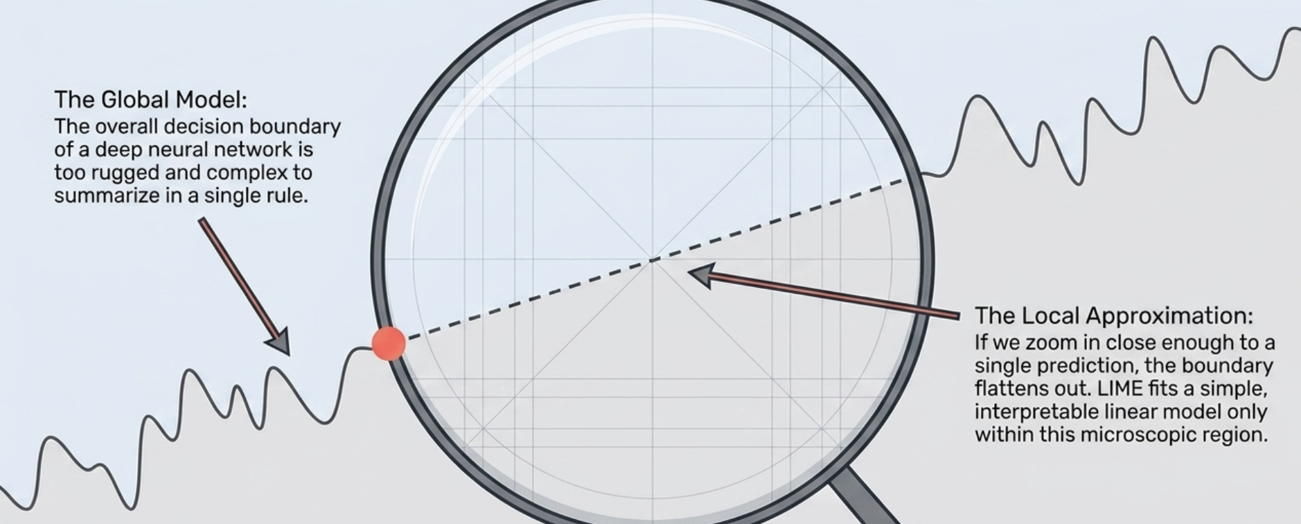 The global decision boundary is too complex to summarise. But zoom in close enough to a single prediction and it flattens out — LIME fits a simple linear model in this microscopic region.
The Algorithm
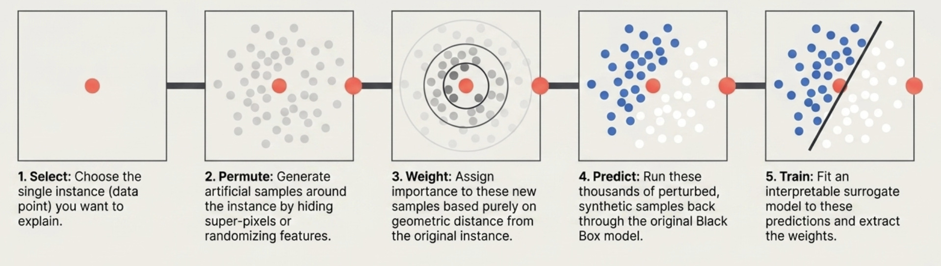 The five-step LIME pipeline: choose an instance, perturb it, weight by proximity, get black-box predictions, fit an interpretable surrogate.
Step 1 – Select the instance. Pick the prediction you want to explain.
Step 2 – Generate perturbations. Create a neighbourhood dataset around the instance. How perturbation works depends on the data type:
- Tabular data: For continuous features, sample from a normal distribution with the same mean and standard deviation as the training data. For categorical features, sample categories proportional to training frequencies. This is not permutation-shuffling – it is generating new synthetic points.
- Text: Randomly remove words from the document. Each perturbation is a subset of the original words, represented as a binary vector (word present or absent).
- Images: Decompose the image into superpixels (contiguous patches of similar pixels, computed via standard segmentation algorithms). Each perturbation turns superpixels on or off – a binary vector over superpixel presence.
Step 3 – Weight by proximity. Not all perturbations matter equally. Samples close to the original instance should influence the local model more. LIME uses an exponential (Gaussian) kernel:
\[\pi_x(z) = \exp\left(-\frac{D(x, z)^2}{\sigma^2}\right)\]where $D$ is a distance function (L2 for images, cosine for text) and $\sigma^2$ is the kernel width. Points far from $x$ get weights near zero; points close to $x$ get weights near one.
Step 4 – Get black-box predictions. Query the original model $f$ on each perturbed sample. These predictions become the labels for training the surrogate.
Step 5 – Fit the interpretable model. Train a weighted linear model (or decision tree) on the perturbed samples, using the black-box predictions as targets and the proximity weights from Step 3.
Step 6 – Interpret. The fitted coefficients of the linear model are the explanation. Large positive weight on a feature means it pushed the prediction toward the class; large negative weight means it pushed away.
The Math
LIME solves the following optimisation:
\[\xi(x) = \underset{g \in G}{\arg\min}\ \mathcal{L}(f, g, \pi_x) + \Omega(g)\]
where:
- $f$ is the black-box model (outputs class probability)
- $G$ is the family of interpretable models (e.g., linear models)
- $\mathcal{L}(f, g, \pi_x)$ measures how unfaithful $g$ is to $f$ in the neighbourhood defined by $\pi_x$
- $\Omega(g)$ penalises complexity (number of non-zero weights for linear models, depth for trees)
For sparse linear explanations, $g(z’) = w \cdot z’$ where $z’ \in {0, 1}^{d’}$ is the interpretable binary representation. The loss becomes a weighted least-squares problem:
\[\mathcal{L}(f, g, \pi_x) = \sum_{z \in \mathcal{Z}} \pi_x(z) \left(f(z) - g(z')\right)^2\]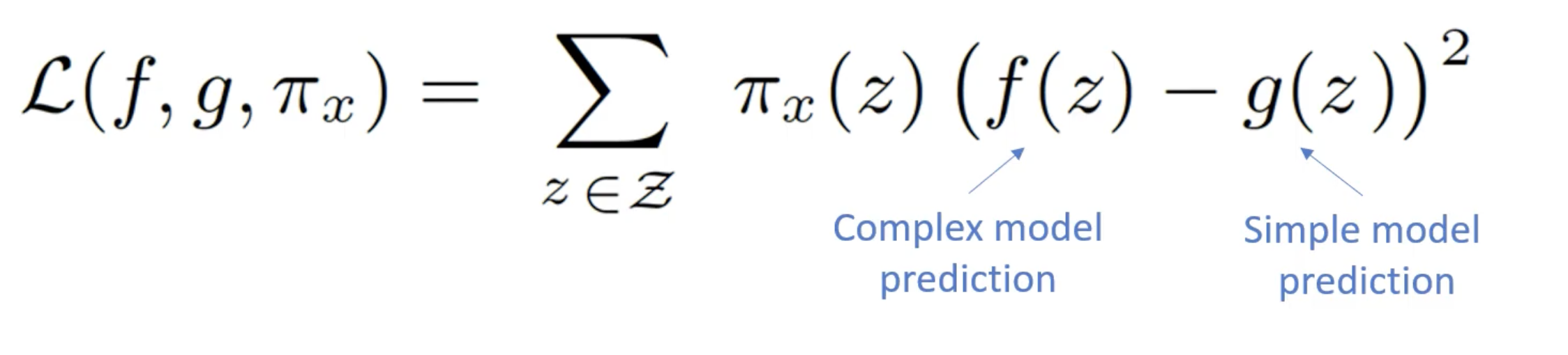 The fidelity term: weighted squared difference between the black-box prediction $f(z)$ and the surrogate $g(z)$, with proximity weights $\pi_x(z)$.
The complexity term enforces sparsity: select at most $K$ features. In practice, LIME uses Lasso with a slowly decreasing regularisation parameter $\lambda$ until exactly $K$ non-zero weights remain. The default in the LIME package is $K = 10$.
The kernel width defaults to $\sigma = 0.75 \sqrt{d’}$ where $d’$ is the number of interpretable features. This controls the “zoom level” – too small and you capture insufficient variation; too large and the linear assumption breaks down.
What Explanations Look Like
Tabular data: Bar charts showing feature contributions. For an abalone ring-count prediction: shell_weight pushed the prediction up, shucked_weight pushed it down. The bars give relative importance – not exact additive contributions.
Text classification: Words highlighted by contribution. A spam classifier might highlight free, click, winner as pushing toward spam. A sentiment model highlights excellent and recommend as positive contributors.
Image classification: Superpixels that support the prediction are shown; the rest are greyed out. For an “electric guitar” prediction, the explanation highlights the guitar body. For “Labrador”, it highlights the dog’s face. If it highlighted the background snow instead, you would know the model learned a spurious correlation (the wolf-vs-husky problem from the original paper).
Limitations
- Instability: Run LIME twice on the same instance with different random perturbations and you may get different explanations. This undermines trust in the explanations themselves.
- Kernel width sensitivity: The choice of $\sigma$ significantly affects results, and there is no principled method to select it for a given problem.
- Superpixel quality: For images, explanation quality depends on the segmentation algorithm. Poor superpixels yield poor explanations.
- Improbable perturbations: Sampling features independently ignores correlations. For tabular data, this generates instances that could never occur in reality (e.g., a 5-year-old with a PhD), yet these unrealistic points influence the local model.
- Local only: LIME explains one prediction. It does not tell you whether the model is generally trustworthy. The paper proposes SP-LIME (Submodular Pick) to select a representative set of explanations that cover the feature space, but this is a heuristic.
- Manipulability: The flexibility in choosing kernel width, number of features, discretisation, and surrogate model means one can tune parameters until a desired explanation appears – a form of explanation hacking.
Key Takeaways
- LIME explains individual predictions of any model by fitting a local interpretable surrogate.
- The core loop: perturb → predict → weight → fit → read coefficients.
- It works across modalities – tabular, text, images – by defining appropriate perturbation and distance functions.
- Explanations are relative feature importances, not exact additive contributions (unlike SHAP).
- Instability and sensitivity to hyperparameters (kernel width, $K$, discretisation) are serious practical concerns.
- Local explanations do not guarantee global model trustworthiness.
Further Reading
- Ribeiro, Singh & Guestrin, “Why Should I Trust You?”: Explaining the Predictions of Any Classifier (2016) – arXiv:1602.04938
- LIME Python package (GitHub)
- Christoph Molnar, Interpretable Machine Learning – Chapter on LIME